Deep Learning for Segmentation of Hyperspectral Satellite Images

Teaching a shoebox-sized satellite to decide what’s worth sending home

A hyperspectral CubeSat sees far more than it can ever transmit. HYPSO-2 orbits at roughly 500 km, captures cubes of over a hundred narrow spectral bands per scene, and gets only a few minutes of ground-station contact per pass. So the question is not can we classify the imagery but can the spacecraft decide, on-board and in real time, which pixels are worth the downlink before the window closes. This project, for the NTNU SmallSat Lab, ports the 1D-JustoLiuNet network from HYPSO-1 to HYPSO-2 so the satellite can label every pixel sea, land, or cloud. The headline is not that the port works on easy data. It is that accuracy falls from 0.96 on near-identical imagery to 0.37 on geographically diverse imagery, and most of the work is diagnosing why.

Why a lab that watches the ocean needs a CNN on-board

HYPSO exists to observe ocean colour: algal blooms, phytoplankton, river plumes. HYPSO-1 launched in 2022 and HYPSO-2 in 2024, both 6U CubeSats with a pushbroom hyperspectral imager and a small FPGA-based processing unit. A hyperspectral cube is enormous and the downlink is tiny, so the satellite has to be selective. A scene that is 90 % cloud is worthless to an oceanographer; a clear stretch of sea carrying a bloom is the whole point of the mission. A per-pixel segmentation running on-board lets the spacecraft make that call itself. The classifier has to be small enough for a modest FPGA and robust enough for the wildly varying scenes a polar orbit sees. This project stress-tests the second requirement.

One pixel, one spectrum, one label

Each image is a cube with two spatial axes and about 112 spectral bands from the visible into the near-infrared. The load-bearing idea behind the whole model family is the spectral-signature assumption: different materials reflect different wavelengths differently, so one pixel’s reflectance curve across a hundred bands is enough to name the material. No spatial context needed.

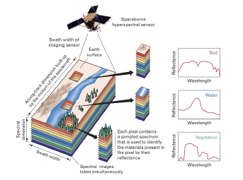
The classifier is therefore a function of the spectrum only, applied independently to every pixel. That single commitment is what the diversity tests put under pressure.

1D-JustoLiuNet. Four Conv1D → ReLU → MaxPool blocks slide learnable band-pass detectors along the spectral axis, widening the channels from 1 to 24 while halving the length each time, then a flatten to 48 features and one linear layer to three logits. Small enough to run pixel by pixel at the spacecraft’s clock rate, which is the point.

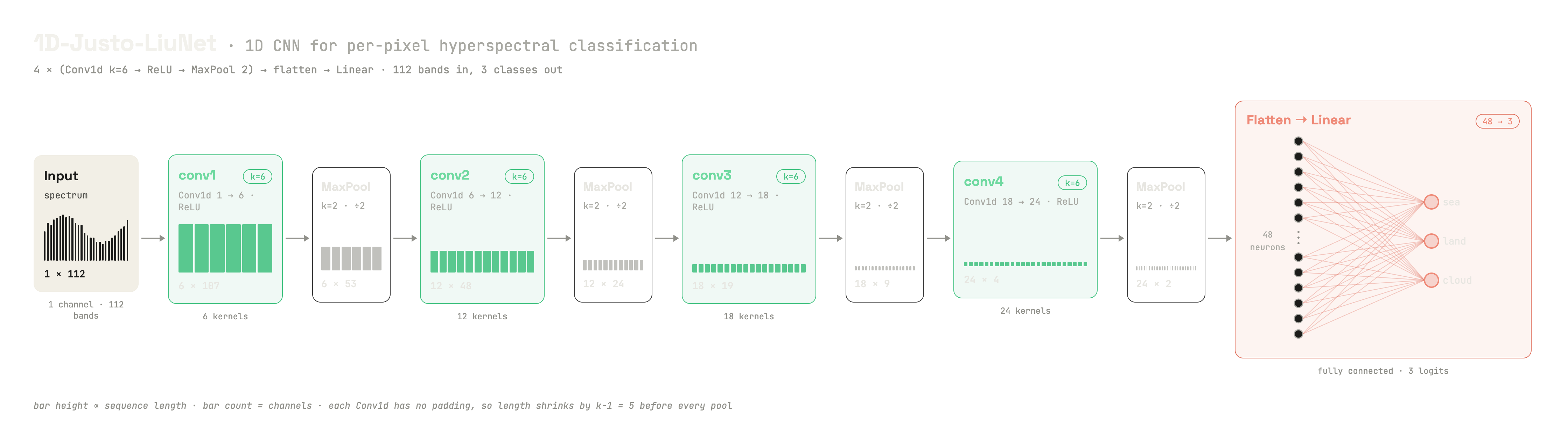
Before a spectrum reaches the network it is min-max normalised per image, per band. Training uses cross-entropy with label smoothing, AdamW, and deliberately conventional hyperparameters, so any pathology is attributable to the architecture or the data rather than the recipe. The published network reaches about 93 % on HYPSO-1; that is the number this project is trying to reach on HYPSO-2.

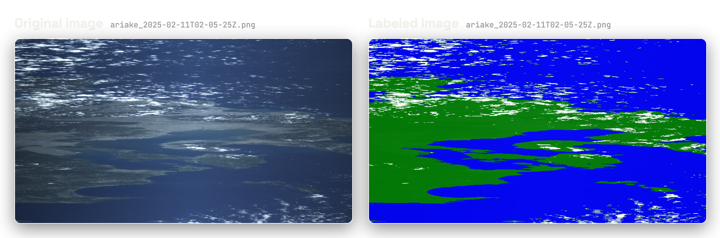
The labels, and their noise. Ground truth is generated semi-automatically in ENVI from spectral thresholds plus manual cleanup. It is not perfect: ENVI routinely mislabels sea pixels near clouds as land.

Results: a clean collapse as the data diversifies

Six controlled tests vary how similar the evaluation images are to the training images, and how homogeneous the dataset is. T01 to T03 are sanity checks, T04 a medium similarity test, and T05 and T06 the hard diversity tests drawn from geographically and environmentally varied imagery: the regime that mirrors deployment.

Test	Type	Difficulty	Images	Sim. index
T01	Sanity	Easy	6	1
T02	Sanity	Easy	8	0
T03	Sanity	Easy	25	1
T04	Similarity	Medium	9	1
T05	Diversity	Hard	12	0
T06	Diversity	Hard	27	0

The degradation is monotonic as the data diversifies:

Test	Accuracy	Weighted $F_1$	Macro $F_1$	Notable failure
T01 (sanity)	$0.81$	$0.80$	$0.54$	cloud $F_1 = 0.01$, class collapse
T02 (sanity)	$0.76$	$0.77$	$0.75$	balanced — best macro-$F_1$
T03 (sanity, replicated image)	$0.96$	$0.95$	$0.40$	majority-class memorisation
T04 (similarity)	$0.63$	$0.61$	$0.41$	cloud $F_1 = 0.00$
T05 (diversity)	$0.42$	$0.39$	$0.35$	sea / land confused
T06 (diversity)	$0.37$	$0.37$	$0.36$	$\approx$ chance for three classes

Two rows matter. T03 trains and evaluates on 25 near-identical frames: accuracy looks spectacular at 0.96, but macro-F1 is 0.40 because the model has memorised the majority class and puts nearly every cloud and sea pixel into “land”. T06 is the deployment regime, and weighted F1 collapses to 0.37, barely above the majority-class baseline. Everywhere, the class with the largest support scores best and the rarest class is dropped first.

Why 37 % and not 93 %. Four factors compound, and architecture is not the dominant one.

• The datasets are not comparable. The published 93 % was measured on a deliberately easy corpus: no snow, little environmental variation, high visual similarity. The diversity tests are the opposite. Most of the gap is a difference in problem difficulty, not model quality.
• Per-image normalisation compresses inter-image variability. Rescaling each image independently flattens the genuine spectral differences between scenes, so a sea pixel from one orbit and one from another can land at similar values even when their raw spectra differ. Standard practice, but here it works against the model.
• Label noise. The Ariake mislabelling is systematic and pulls the boundaries off. A real contributor, but it cannot account for a 56-point gap on its own.
• Class imbalance and no regularisation. Cross-entropy favours the majority class unless reweighted, and with plain ReLU and no dropout the network is free to memorise. The widening train-versus-eval gap on T05 and T06 is the fingerprint.

What I took away

The accuracy number a paper reports is inseparable from the dataset it was measured on, and a model that classifies one pixel from its spectrum alone has no way to recover when the spectra themselves drift between scenes. The fixes follow from the diagnosis: normalise across the corpus rather than per image, reweight or resample the rare classes, add dropout, and, more fundamentally, let the model see a pixel’s neighbourhood. Each of them is a test away.