Back to all projects

Feb 2026 – May 2026

AI · SWE

Last edited

Compositional Analysis for Safety Specifications

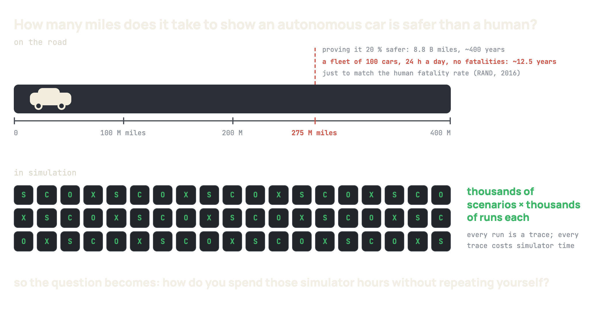
This project extends compositional statistical model checking for autonomous vehicles from Markovian to non-Markovian safety specifications.

The core idea is to augment simulation states with DFA states that encode the temporal logic of the specification, then propagate the DFA distribution across primitive scenario traces. This makes it possible to verify safety properties that depend on the history of events (not just the current state) while preserving the compositional structure that keeps large-scale verification tractable.

Affiliation

UC Berkeley

Partners

Report

  • Manuscript

Keywords

  • Compositional Analysis
  • Statistical Model Checking
  • DFA
  • Automata Theory
  • Markov Chains
  • Python
  • VerifAI
  • MetaDrive
  • CARLA
  • Webots
  • Scenic

Deepdive

Introduction

This project extends VerifAI’s compositional statistical model checking (SMC) from Markovian to non-Markovian safety specifications, and adds a Scenic frontend so that composite driving scenarios written in standard Scenic source can be analyzed end-to-end. Compositional analysis decomposes a long simulation into short primitive scenarios whose traces are generated in parallel and stitched together via importance sampling at handoff boundaries; the contribution here is representing each safety property as a deterministic finite automaton (DFA) and propagating a distribution over DFA states across those handoffs so that history-dependent properties, “stop at most once at a tollgate,” “once the vehicle exceeds 15 m/s it must never drop below 6.5 m/s”, fall inside the compositional framework. On the MetaDrive simulator and on a Scenic intersection benchmark, the framework recovers monolithic estimates to within statistical error while achieving a 4–7× wall-clock speedup.

This was a joint course project for EECS 219C (Formal Methods: Specification, Verification, and Synthesis) at UC Berkeley, Spring 2026, with Abhi Pomalapally. Abhi led the VerifAI backend (DFA-augmented state-distribution propagation, the rejection-conditioning fix in check_with_dfa, and the MetaDrive evaluation); I led the Scenic frontend (the recursive DAG parser over containers, composition statements, and weighted invocations, and the linearization that feeds the backend); Abhi also handled the end-to-end Scenic → MetaDrive integration.

Problem Definition

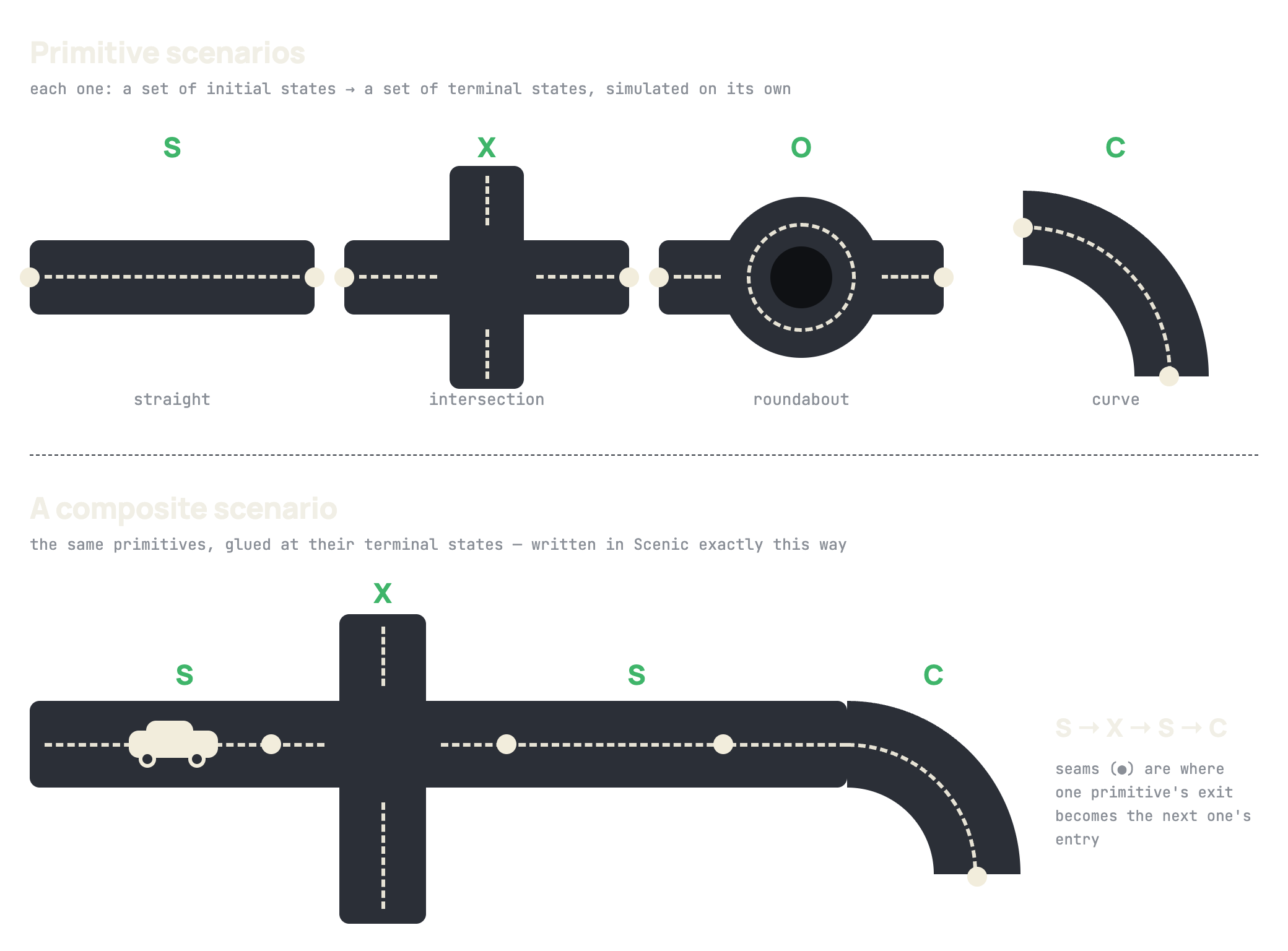
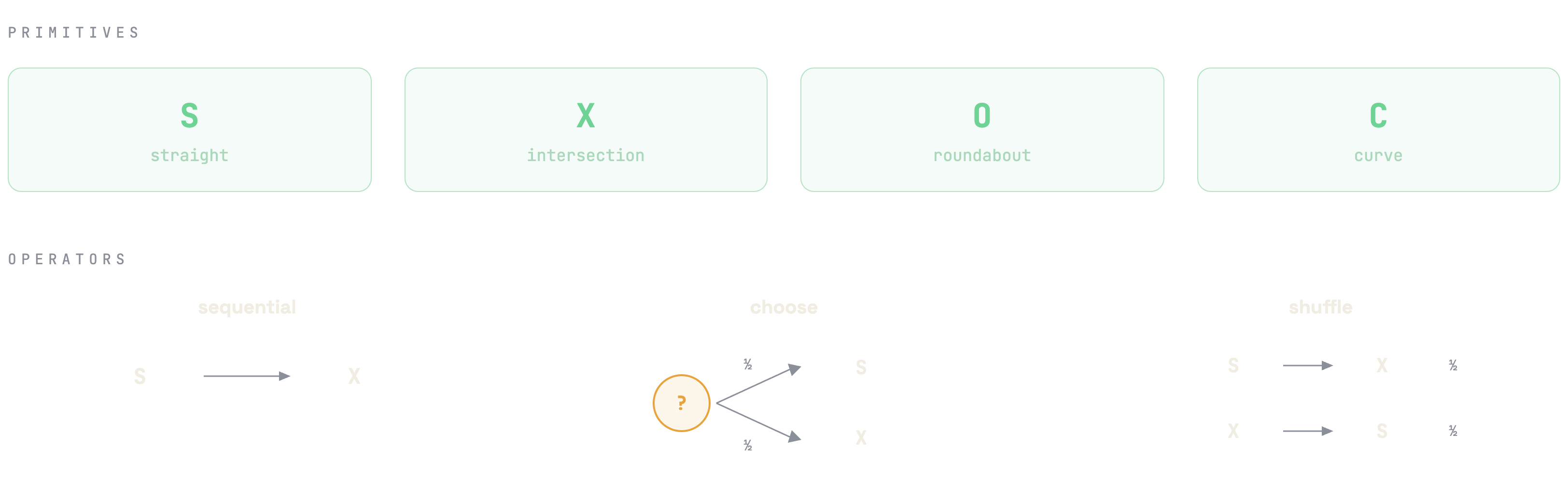
Primitive and composite scenarios. Let S\mathcal{S} denote a finite set of primitive scenarios. Each primitive sSs \in \mathcal{S} induces a Markov decision process Ms=(X,A,Ps,x0s)M_s = (X, A, P_s, x_0^s) with shared state space XX, action space AA, transition kernel PsP_s, and initial state x0sx_0^s. Under the system policy, MsM_s yields traces τ=(x0,x1,,xT)\tau = (x_0, x_1, \dots, x_T) distributed according to some trace distribution Ds\mathcal{D}_s. A composite scenario cc is built from primitives via three composition operators, mirroring Scenic’s do, do choose, and do shuffle clauses:

  • sequential composition c1;c2c_1 ; c_2, which runs c1c_1 to its terminal state and then c2c_2 from that state;
  • probabilistic choice choose{(c1,w1),,(ck,wk)}\textsf{choose}\{(c_1, w_1), \dots, (c_k, w_k)\}, which executes cic_i with probability wi/jwjw_i / \sum_j w_j;
  • shuffle shuffle{c1,,ck}\textsf{shuffle}\{c_1, \dots, c_k\}, which executes the cic_i‘s in a uniformly random order.

Specifications and satisfaction probability. A specification φ\varphi is given by a deterministic finite automaton Aφ=(Q,Σ,δ,q0,F)\mathcal{A}_\varphi = (Q, \Sigma, \delta, q_0, F) together with a labeling function L:XΣL : X \to \Sigma. A trace τ=(x0,,xT)\tau = (x_0, \dots, x_T) satisfies φ\varphi, written τφ\tau \models \varphi, iff the run q0,q1,,qTq_0, q_1, \dots, q_T given by qt+1=δ(qt,L(xt+1))q_{t+1} = \delta(q_t, L(x_{t+1})) ends in an accepting state, qTFq_T \in F. The quantity of interest is

ρ(c,φ)  =  PrτDc[τφ].\rho(c, \varphi) \;=\; \Pr_{\tau \sim \mathcal{D}_c}[\tau \models \varphi].

We call φ\varphi Markovian if τφ\tau \models \varphi depends only on the terminal state xTx_T, and non-Markovian otherwise.

The compositional non-Markovian analysis problem. Given a composite scenario cc over primitives S\mathcal{S}, a non-Markovian specification φ\varphi given by (Aφ,L)(\mathcal{A}_\varphi, L), and a per-primitive simulation budget of NN traces, produce an estimate ρ^(c,φ)\hat{\rho}(c, \varphi) of ρ(c,φ)\rho(c, \varphi) with a confidence half-width ε^\hat{\varepsilon} at level δ\delta (so that ρ^,ρε^|\hat{\rho}, \rho| \leq \hat{\varepsilon} holds with probability at least 1,δ1, \delta), using only the primitive trace sets {τis}i=1NDs\{\tau_i^s\}_{i=1}^N \sim \mathcal{D}_s for sSs \in \mathcal{S}.

Why the problem is hard. The restriction to primitive traces is what makes the problem useful, primitives are short, can be simulated in parallel, and need not be re-run when cc changes, and also what makes it technically nontrivial. First, since φ\varphi may be non-Markovian, ρ(c,φ)\rho(c, \varphi) depends on the full trace rather than its terminal state, which rules out the Markovian compositional estimator of Yalcinkaya et al. (RV 2023). Second, in c1;c2c_1 ; c_2, the state distribution at the end of c1c_1 generally differs from the initial-state distribution of c2c_2 when c2c_2 is simulated as a primitive, so naively concatenating primitive traces yields a biased estimate of ρ(c1;c2,φ)\rho(c_1 ; c_2, \varphi) unless this mismatch is explicitly corrected.

Approach

Given a composite Scenic program cc and a non-Markovian specification φ=(Aφ,L)\varphi = (\mathcal{A}_\varphi, L), the framework returns (ρ^(c,φ),ε^)(\hat{\rho}(c, \varphi), \hat{\varepsilon}) in four stages: (i) recursively parse the Scenic source into a composition graph over primitives S\mathcal{S}; (ii) simulate NN traces per primitive in parallel; (iii) walk the graph, propagating a distribution over DFA states and correcting trace-distribution mismatch with kernel-density importance sampling; (iv) aggregate sibling branches by operator (product for sequential, weighted mixture for choose, permutation average for shuffle).

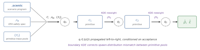
End-to-end pipeline: a Scenic source, a DFA safety spec, and primitive trace pools feed an initial DFA-state distribution q0, which is propagated left-to-right across primitives c1, c2, ..., with a KDE reweight at each boundary, producing the estimate and confidence half-width.
End-to-end pipeline. Three inputs (left) feed the framework: the Scenic source .scenic, the DFA safety spec Aφ\mathcal{A}_\varphi, and per-primitive trace pools {Ts}\{\mathcal{T}_s\}. The frontend parses the source into a linearized composition CC; the backend propagates the DFA-state distribution q0q1q2q_0 \to q_1 \to q_2 left-to-right conditioned on acceptance, with a KDE reweight at each boundary, producing (ρ^,ε^)(\hat{\rho}, \hat{\varepsilon}).

Scenic Frontend

Scenic’s composition vocabulary (do, do choose, do shuffle, and nested scenario blocks) maps directly onto the sequential, probabilistic-choice, and shuffle operators above, so a Scenic program already carries the compositional decomposition the analysis needs. The challenge is that composition in Scenic nests arbitrarily: a compose block can invoke another scenario whose body has further choose or shuffle clauses, and nested choose weights combine multiplicatively along invocation paths. For example, choose{A:0.5,M:0.5}\textsf{choose}\{A{:}0.5, M{:}0.5\} with M=choose{B:0.6,C:0.4}M = \textsf{choose}\{B{:}0.6, C{:}0.4\} is the three-way distribution (A:0.5,B:0.3,C:0.2)(A{:}0.5, B{:}0.3, C{:}0.2), not the two-way (A:0.5,M:0.5)(A{:}0.5, M{:}0.5) obtained by reading the outer choose in isolation. A flat parse loses this structure; recovering Dc\mathcal{D}_c requires a recursive traversal of the Scenic abstract syntax tree (AST) that preserves operator semantics and propagates weights across invocation boundaries.

A Scenic source with a nested choose on the left, and its extracted composition DAG on the right. The DAG has container nodes, statement nodes (do, do choose, do shuffle), and invocation nodes connected by contains, invokes, and next edges.
Scenic source with a nested choose (left) and its extracted composition DAG (right). All three node kinds (VCV_C containers, VSV_S statements, VIV_I invocations) and all three edge kinds (contains, invokes, next) are exercised.

The composite scenario is represented as a directed acyclic graph G=(V,E)G = (V, E) with V=VCVSVIV = V_C \cup V_S \cup V_I partitioned into three node kinds. VCV_C contains one container node per scenario or behavior definition; VSV_S contains one statement node per do, do choose, or do shuffle clause, each carrying its operator label; VIV_I contains one invocation node per call site, each carrying a target identifier and (under choose) a positive weight. Edges fall into three kinds: contains (a container to each of its statements), invokes (a statement to its invocations and each invocation to its target), and next (between sibling statements inside a container, encoding sequential order).

The DAG is then linearized into a list of CompositionStep values, where

CompositionStep  =  S    {f:S[0,1]    sSf(s)=1}.\textsf{CompositionStep} \;=\; \mathcal{S} \;\cup\; \Bigl\{ f : \mathcal{S} \to [0, 1] \;\Big|\; \textstyle\sum_{s \in \mathcal{S}} f(s) = 1 \Bigr\}.

Sequential statements concatenate their children’s step lists; choose produces a single step that flattens the child step lists into a distribution by multiplying weights along the invocation path; shuffle over kk children yields the k!k! permutation step lists with uniform weight 1/k!1/k!.

VerifAI Backend

The backend extends VerifAI’s compositional analysis engine from the Markovian estimator of Yalcinkaya et al. to DFA safety specifications. A new automaton_specification class in VerifAI wraps the dfa library to represent a safety property as Aφ=(Q,Σ,δ,q0,F)\mathcal{A}_\varphi = (Q, \Sigma, \delta, q_0, F) with labeling L:XΣL : X \to \Sigma, and extends the engine to consume it. It takes the linearized composition C=(c1,,cN)C = (c_1, \dots, c_N) from the frontend, where each cic_i is either a primitive name (sequential step) or a weighted dictionary {s(j):pj}j\{s^{(j)} : p_j\}_j (random choice), along with the per-primitive trace pools Ts\mathcal{T}_s and entry/exit features ϕsrc,ϕtgt\phi_{\text{src}}, \phi_{\text{tgt}} (e.g., position, speed), and returns (ρ^,ε^)(\hat{\rho}, \hat{\varepsilon}) estimating Pr[δ^(q0,L(τ))F]\Pr[\hat{\delta}(q_0, L(\tau)) \in F] over the composite distribution.

Example DFA for the safety spec 'no more than one near-stop' with three states: moving (start), stopped_once, and stopped_twice (absorbing rejecting). near_stop transitions advance the count; the absorbing state is reached after a second near_stop.
Example DFA for the safety spec “no more than one near-stop.” stopped_twice is absorbing rejecting.

Three challenges shape the algorithm.

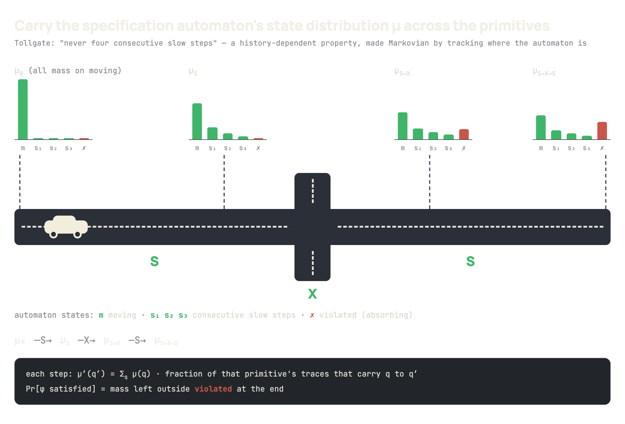
Non-Markovian satisfaction. The Markovian estimator labels each trace by 1[L(xT)]\mathbf{1}[L(x_T)]; DFA satisfaction instead depends on the full labeled sequence and on the entry state. We maintain a distribution qdist(i)Δ(Q)q_{\text{dist}}^{(i)} \in \Delta(Q) over DFA entry states, conditioned across primitives on acceptance, and label each trace by

i(τ)  =  qQqdist(i)(q)1 ⁣[δ^(q,L(τ))F].\ell_i(\tau) \;=\; \sum_{q \in Q} q_{\text{dist}}^{(i)}(q)\, \mathbf{1}\!\bigl[\hat{\delta}(q, L(\tau)) \in F\bigr].

The accept-conditioning is essential: advancing qdist(i)q_{\text{dist}}^{(i)} over all step-ii traces (including ones already in absorbing rejecting states) deflates both ρ^i\hat{\rho}_i and ρ^i+1\hat{\rho}_{i+1}, so iρ^i\prod_i \hat{\rho}_i underestimates the truth. We therefore compute the full sequence {qdist(i)}i=1N\{q_{\text{dist}}^{(i)}\}_{i=1}^N in a forward pass over CC before the main estimation loop, so each step uses the correct pre-step distribution.

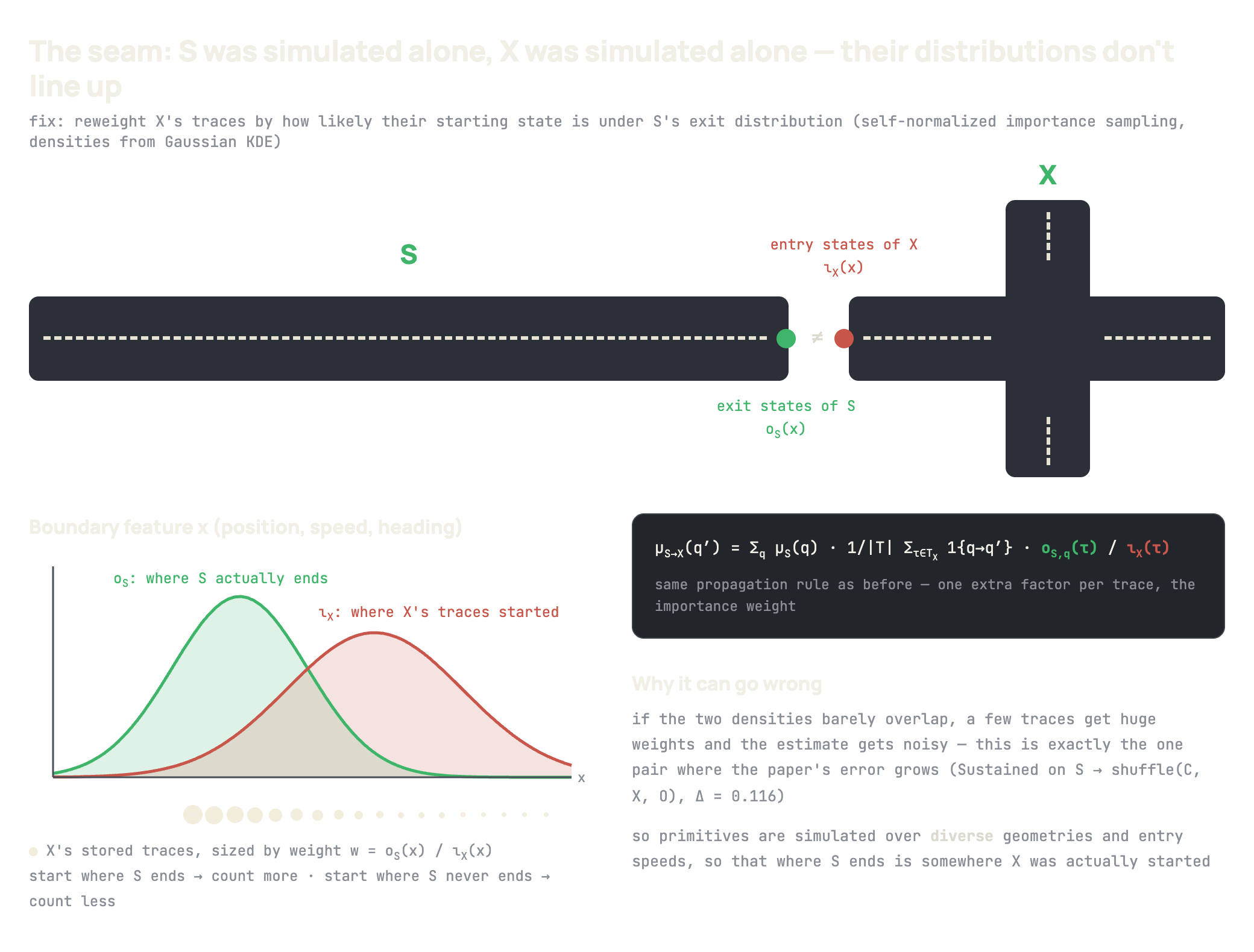
Handoff distribution mismatch. Each primitive is simulated standalone, so its entry distribution over XX differs from its predecessor’s exit distribution; naive concatenation is biased. We correct with self-normalized importance sampling: fit a Gaussian KDE psrc(i)p_{\text{src}}^{(i)} to step i1i{-}1‘s accepting-exit features ϕtgt\phi_{\text{tgt}} and ptgt(i)p_{\text{tgt}}^{(i)} to step ii‘s entry features ϕsrc\phi_{\text{src}}, with

w~i(τ)  =  psrc(i)(ϕsrc(τ))ptgt(i)(ϕsrc(τ)),wi(τ)  =  w~i(τ)/τw~i(τ).\tilde{w}_i(\tau) \;=\; \frac{p_{\text{src}}^{(i)}(\phi_{\text{src}}(\tau))}{p_{\text{tgt}}^{(i)}(\phi_{\text{src}}(\tau))}, \qquad w_i(\tau) \;=\; \tilde{w}_i(\tau) \,/\, {\textstyle\sum_{\tau'}} \tilde{w}_i(\tau').

The per-step estimate is the self-normalized IS-weighted mean ρ^i=τw~i(τ)i(τ)/τw~i(τ)\hat{\rho}_i = \sum_\tau \tilde{w}_i(\tau)\, \ell_i(\tau) / \sum_\tau \tilde{w}_i(\tau). Near-disjoint supports collapse the weights, which we mitigate by prewarming primitives so successive supports overlap, and by monitoring effective sample size.

Random-choice composition. A step ci={s(j):pj}jc_i = \{s^{(j)} : p_j\}_j branches all three machinery components:

ρ^i  =  jpjρ^i,j,qdist(i+1)  =  jpjq~dist(i+1),j,\hat{\rho}_i \;=\; \sum_j p_j\, \hat{\rho}_{i,j}, \qquad q_{\text{dist}}^{(i+1)} \;=\; \sum_j p_j\, \tilde{q}_{\text{dist}}^{(i+1), j},

where ρ^i,j\hat{\rho}_{i,j} is the per-branch IS estimate from a shared qdist(i)q_{\text{dist}}^{(i)} and q~dist(i+1),j\tilde{q}_{\text{dist}}^{(i+1), j} is its accept-conditioned successor. When step i+1i{+}1 fits its source KDE, accepting-exit features are pooled across branches with weights pj\propto p_j, so the mixture mass is faithful rather than implicitly uniform.

Aggregation

The chain rule

Pr[i=1Naccepti]  =  i=1NPr[acceptiaccept<i]\Pr\Bigl[\bigwedge_{i=1}^N \text{accept}_i\Bigr] \;=\; \prod_{i=1}^N \Pr[\text{accept}_i \mid \text{accept}_{<i}]

justifies multiplying per-step estimates into the composite estimate, with per-step Hoeffding bounds ε^i\hat{\varepsilon}_i (using the effective sample size NeffN_{\text{eff}} of the importance weights) propagated as

ρ^  =  i=1Nρ^i,ε^  =  ρ^i=1N(ε^i/ρ^i)2,ε^i2  =  jpj2ε^i,j2.\hat{\rho} \;=\; \prod_{i=1}^N \hat{\rho}_i, \qquad \hat{\varepsilon} \;=\; \hat{\rho}\sqrt{{\textstyle\sum_{i=1}^N} (\hat{\varepsilon}_i / \hat{\rho}_i)^2}, \qquad \hat{\varepsilon}_i^2 \;=\; {\textstyle\sum_j} p_j^2\, \hat{\varepsilon}_{i,j}^2.

A union bound over the NN per-step events with δi=δ/N\delta_i = \delta / N ensures the composite estimate holds at overall confidence 1,δ1, \delta.

Results

We evaluate accuracy and efficiency against the monolithic SMC baseline (which simulates each composite as a single chained Scenic scenario) on three sets of scenarios in MetaDrive.

Accuracy at matched trace budget

Set A consists of five sequential composites {SX,SXS,SC,SCS,SCX}\{\text{SX}, \text{SXS}, \text{SC}, \text{SCS}, \text{SCX}\} over the primitives Straight, Intersection, Curve, evaluated under two DFAs: φtoll\varphi_{\text{toll}} (rejects after the third near-stop) and φstop\varphi_{\text{stop}} (at most one near-stop). At a matched trace budget, the two estimators agree within Hoeffding intervals on every (c,φ)(c, \varphi) pair.

movingwait₁wait₂wait₃violatedslowslowslowslow (from wait₃ → moving)fast (self)fast (from any waitᵢ)
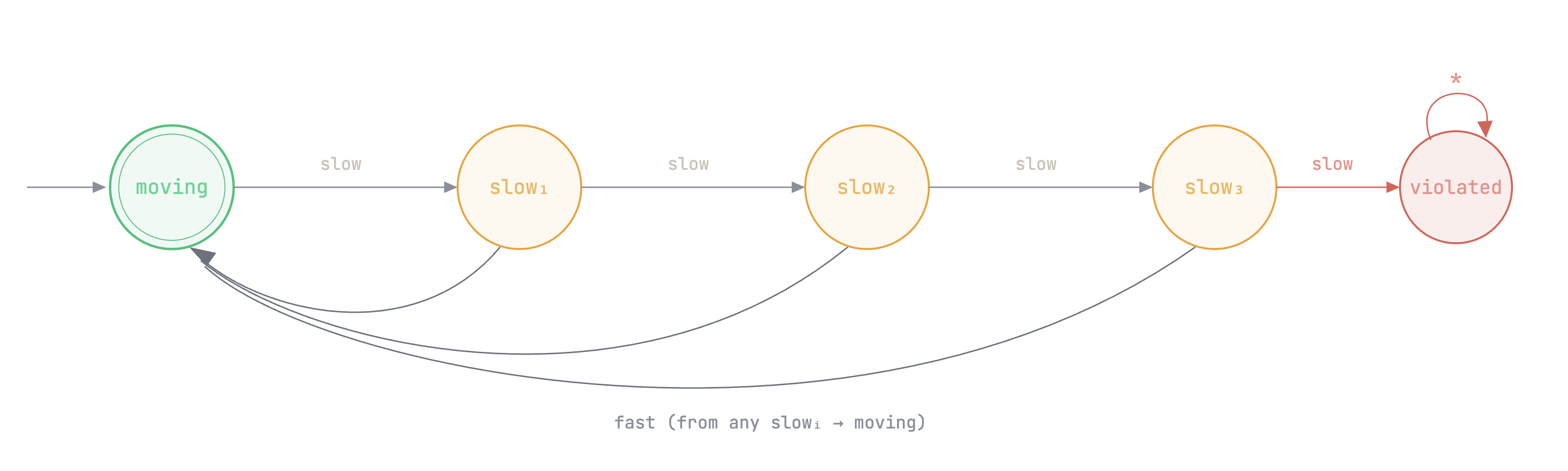
The φtoll\varphi_{\text{toll}} DFA with K=3K{=}3. Slowing down advances the wait counter; resuming speed from any wait state before three consecutive slow steps is a violation; from wait₃, one more slow step returns to moving (the tollgate is cleared). violated is absorbing rejecting.
Compositeρ^mono\hat{\rho}_{\text{mono}} (φtoll\varphi_{\text{toll}})ρ^comp\hat{\rho}_{\text{comp}} (φtoll\varphi_{\text{toll}})ρ^mono\hat{\rho}_{\text{mono}} (φstop\varphi_{\text{stop}})ρ^comp\hat{\rho}_{\text{comp}} (φstop\varphi_{\text{stop}})
SX0.702±0.0610.702 \pm 0.0610.727±0.0920.727 \pm 0.0920.650±0.0610.650 \pm 0.0610.692±0.0970.692 \pm 0.097
SXS0.664±0.0610.664 \pm 0.0610.713±0.1080.713 \pm 0.1080.600±0.0610.600 \pm 0.0610.687±0.1140.687 \pm 0.114
SC0.860±0.0610.860 \pm 0.0610.895±0.0980.895 \pm 0.0980.874±0.0610.874 \pm 0.0610.904±0.1050.904 \pm 0.105
SCS0.862±0.0610.862 \pm 0.0610.892±0.1230.892 \pm 0.1230.866±0.0610.866 \pm 0.0610.897±0.1290.897 \pm 0.129
SCX0.620±0.0610.620 \pm 0.0610.652±0.1010.652 \pm 0.1010.584±0.0610.584 \pm 0.0610.633±0.1040.633 \pm 0.104
Set A on MetaDrive, ρ^±ε^\hat{\rho} \pm \hat{\varepsilon} at δ=0.05\delta = 0.05. Every Δρ^|\Delta\hat{\rho}| falls inside ε^mono+ε^comp\hat{\varepsilon}_{\text{mono}} + \hat{\varepsilon}_{\text{comp}}, i.e. the two estimators agree within statistical error on every (c,φ)(c, \varphi) pair.

Set B is the five-step wander composite Main=5×choose{GoStraight,TurnLeft,TurnRight,Brake}\textsf{Main} = 5 \times \textsf{choose}\{\textsf{GoStraight}, \textsf{TurnLeft}, \textsf{TurnRight}, \textsf{Brake}\}, yielding 45=10244^5 = 1024 distinct execution paths over four leaf primitives. Under φbrake\varphi_{\text{brake}} (rejects after the second hard brake), the compositional estimate ρ^comp=0.868±0.051\hat{\rho}_{\text{comp}} = 0.868 \pm 0.051 agrees with ρ^mono=0.896±0.043\hat{\rho}_{\text{mono}} = 0.896 \pm 0.043, with Δρ^=0.028|\Delta\hat{\rho}| = 0.028 well inside both Hoeffding intervals. The same Set B primitive trace pool was additionally evaluated against seven further DFAs (including non-Markovian properties like rise_then_fall, k_consec_slow, at_most_one_brake) at ~1 s of post-hoc Python each, illustrating that compositional analysis decouples specifications from simulation.

Compositional point estimates land slightly above the monolithic baseline on Set A across all five composites, but the gap is within Hoeffding error in every row and shows no trend with composite length. This is evidence that the accept-conditioning fix in the backend is removing the dominant source of compositional drift, since residual multiplicative bias from un-conditioned rejection mass would grow with the number of primitives.

Efficiency at matched wall-clock budget

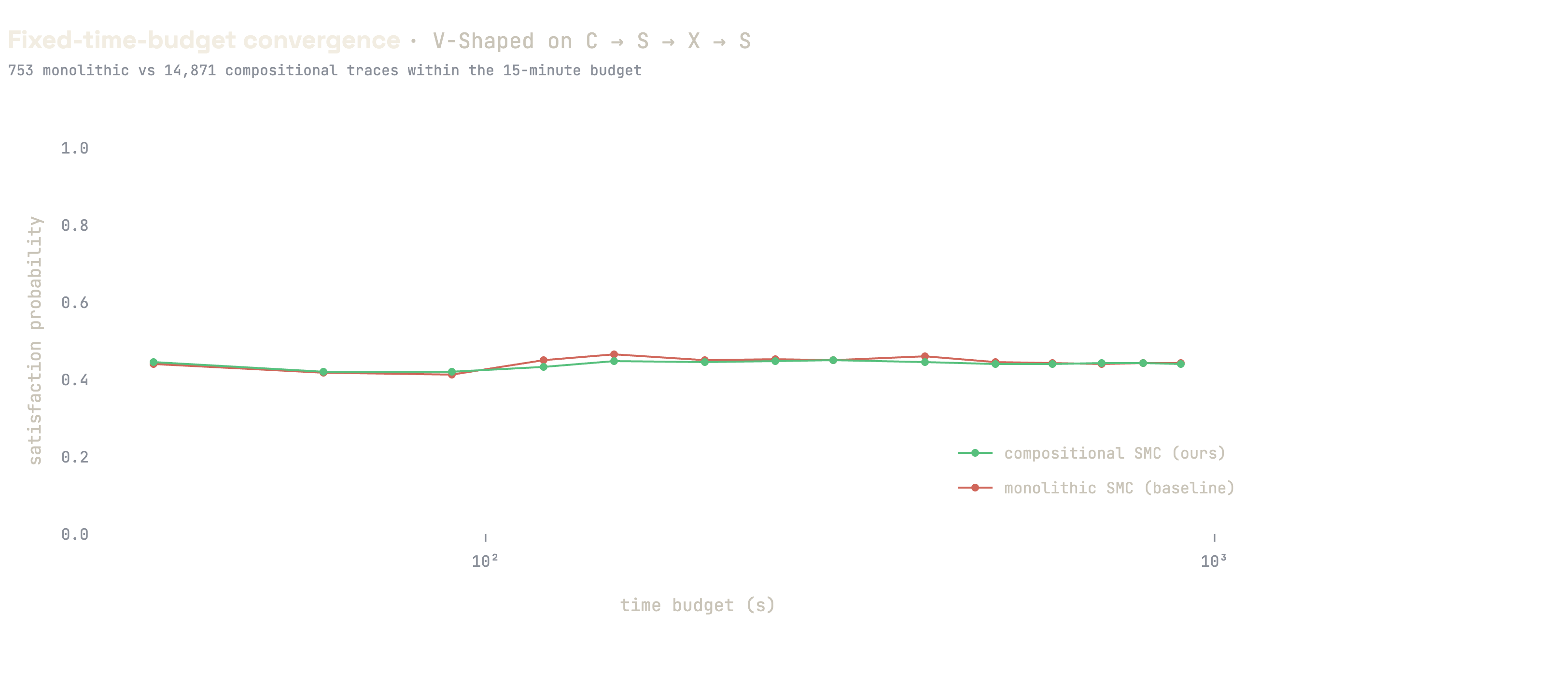
Set C is the two-step approach-then-turn composite Sub1;choose{Sub2L,Sub2R,Sub2S}\textsf{Sub}_1 ; \textsf{choose}\{\textsf{Sub}_2^L, \textsf{Sub}_2^R, \textsf{Sub}_2^S\}, evaluated under the Markovian safe_under_max spec to isolate the wall-clock comparison. Each method runs one continuous simulation up to Tmax=1800sT_{\max} = 1800\,\text{s} and records per-primitive trace counts every ΔT=30s\Delta T = 30\,\text{s}.

Set C wall-clock sweep. Left: Hoeffding half-width epsilon-hat as a function of wall-clock budget T on log-log axes; the compositional curve sits strictly below the monolithic curve at every checkpoint past the simulator startup window. Right: rho-hat with shaded confidence band; both methods agree throughout, so the precision advantage is not bought through bias.
Set C wall-clock sweep under the safe_under_max DFA. Left: ε^\hat{\varepsilon} vs. wall-clock budget TT, log-log. Past the simulator startup window the compositional curve sits strictly below the monolithic curve, with a log-log offset ranging from 4× at ε^=0.20\hat{\varepsilon}^\ast = 0.20 to 7× at ε^=0.15\hat{\varepsilon}^\ast = 0.15. Right: ρ^\hat{\rho} with ±ε^\pm \hat{\varepsilon} band as a function of TT. The two point estimates agree within their confidence intervals throughout, so the precision advantage is not bought through bias.

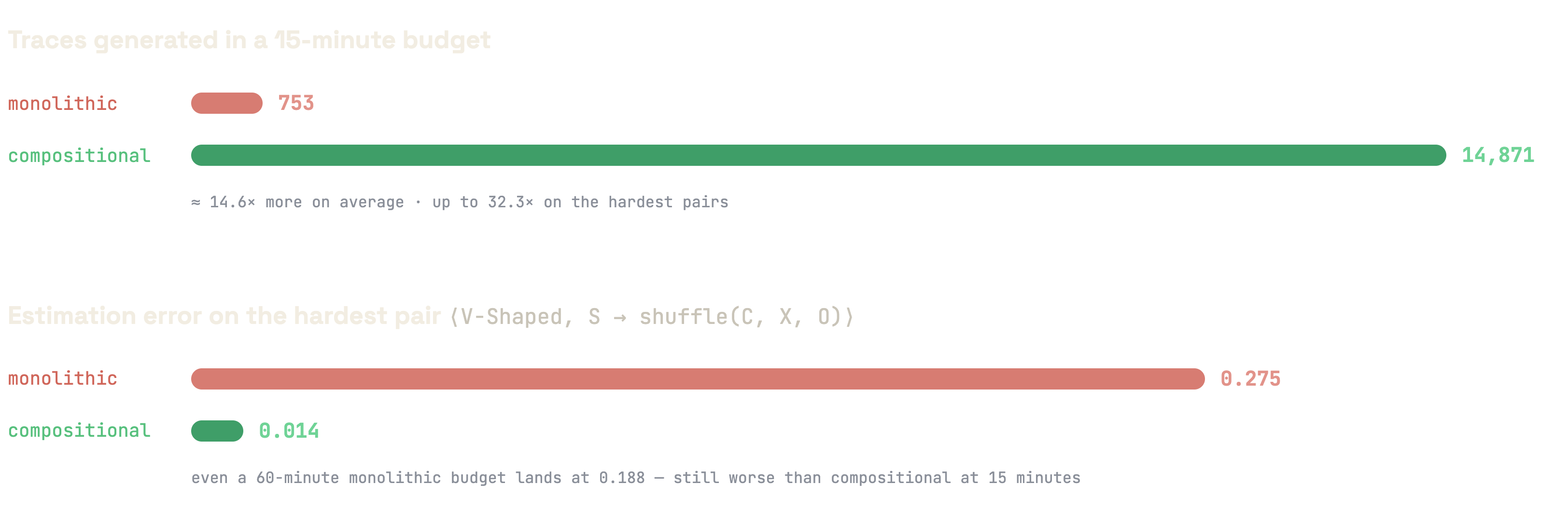
Reading the wall-clock ratio Tmono/TcompT_{\text{mono}} / T_{\text{comp}} at fixed target precision off the left panel yields ≈ 4× at ε^=0.20\hat{\varepsilon}^\ast = 0.20 and ≈ 7× at ε^=0.15\hat{\varepsilon}^\ast = 0.15. Two structural advantages drive this. First, the compositional pipeline spawns one parallel worker per primitive (Sub1\textsf{Sub}_1 together with the three turning branches, four workers in total), while the monolithic pipeline runs a single worker on the chained behavior. Second, each primitive trace covers only one composition step and is therefore a factor of two shorter than a chained composite trace under matched horizons. A third structural advantage, trace-pool reuse across composites sharing the same primitives, is not exercised in this single-composite sweep but would compound the gap on a corpus of composites built from overlapping primitive sets.

Future Work

The framework as it stands handles flat safety DFAs, automata with an absorbing rejecting state where, once acceptance is lost, it cannot be recovered. The natural next step is bounded liveness via complementation: on finite traces of length TT, a bounded-liveness property such as “the vehicle must exceed vmaxv_{\max} at some point” equals 1,ρ(¬φ)1, \rho(\neg\varphi), where ¬φ\neg\varphi is the flat safety property “the vehicle never exceeds vmaxv_{\max} within the trace.” Appendix B of the report validates this empirically on a 4-way intersection composite (ρ^live=0.586±0.060\hat{\rho}_{\text{live}} = 0.586 \pm 0.060 vs monolithic 0.607±0.0780.607 \pm 0.078), confirming the trick is sound when the negation is itself a flat safety DFA. This works because the DFA has only two states and bad is absorbing, so φsafe\varphi_{\text{safe}} collapses to Markovian on the raw simulation state.

The trick does not generalize beyond the bounded-reachability fragment. Bounded-response (“within kk steps of AA, observe BB”), bounded-sequenced-reachability, bounded-persistence, and bounded-recurrence all negate to formulas with nested temporal operators rather than flat safety DFAs, and so cannot be reduced to a single absorbing-reject monitor. Compositional treatment of those classes requires either a product construction across multiple “live” DFA regions or, in the unbounded case, reasoning about infinite-suffix acceptance. A near-term path that stays within the present machinery is bounded response, which is expressible as a finite-window safety DFA and captures a large fraction of practical AV requirements without leaving the absorbing-reject framework.

Two further directions follow naturally. The current implementation lives as an extension of CompositionalAnalysisEngine; upstreaming the DFA monitor and Scenic parser into VerifAI proper would expose them to the existing falsifier pipeline. And the boundary-distribution overlap that compositional estimation requires is currently tuned by hand (spawn-distance and initial-speed calibration on Set A, randomized cruise prewarm on Set B); a diagnostic based on per-handoff effective sample size, paired with an automatic spawn/prewarm adjustment, would remove the manual calibration step and make the framework usable on new primitive libraries without per-scenario tuning.