Tagging the Positron Sky: A Naive Bayes Classifier for β+ Decay

A β⁺ decay ejects a positron that annihilates with an electron into two back-to-back 511 keV photons — the Joliot-Curies' 1934 discovery, and the origin of the Galaxy's brightest gamma-ray line, whose dominant source is still unknown. COSI, a NASA Small Explorer mission launching in 2027, will map that line with high-purity germanium detectors. But the spacecraft is itself activated into a 511 keV background, and COSI's analysis chain had no way to tag β⁺ events; pipelines only ever vetoed them.

BEvAn (the β⁺ Decay Event Analyzer) inverts that test. It reduces each reconstructed event to three physics factors — energy consistency with the 511 keV line, an angular resolution measure of the Compton scatter, and a back-to-back score for the two-photon vertex — and combines them through naive Bayes into a posterior probability of β⁺ origin.

Across seven simulated HPGe geometries differing thirtyfold in detector count, ROC-AUC spans just 98.3–99.6 %. Tuned for completeness, it recovers roughly 90–97 % of true β⁺ events at 80–85 % precision, beats the whole-event 511 keV cut in every geometry, and is a 25 kB model cheap enough to refit as the in-orbit background drifts.

Affiliation

NASA Small Explorers (SMEX) Program / UC Berkeley Space Sciences Laboratory

Partners

Report

In preparation — targeting the American Astronomical Society (AAS)

Keywords

Naive Bayes Classifier
Event Reconstruction
Gamma-Ray Astrophysics
Compton Physics
High-Purity Germanium Detectors
Physics-Informed Machine Learning
Lightweight Models
Python
C++
PyTorch
MEGAlib
Geant4
ROOT

Telling a positron’s death from everything that imitates it

In 1934 the Joliot-Curies bombarded aluminium with alpha particles and made the first artificial radioisotope — phosphorus-30, a β⁺ emitter. A positron does not last long: it stops in matter, meets an electron, and the pair leaves as two 511 keV photons flying apart back-to-back.

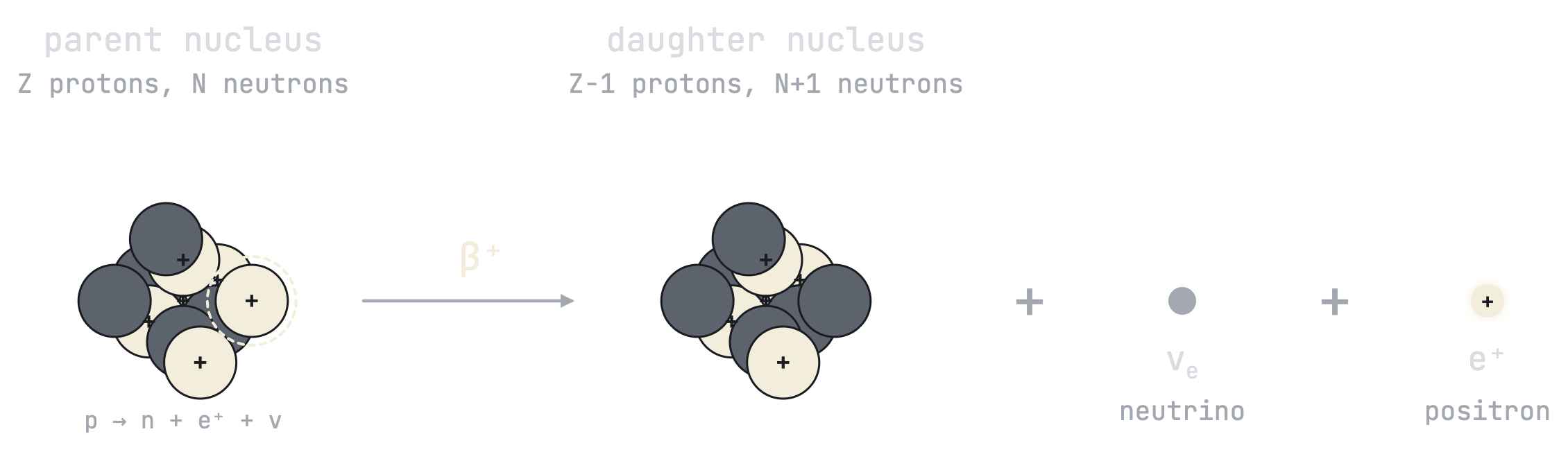
A diagram of beta-plus decay. A parent nucleus with Z protons and N neutrons, one proton highlighted, becomes a daughter nucleus with Z minus 1 protons and N plus 1 neutrons, plus an electron neutrino and a positron. The reaction p → n + e⁺ + ν is written beneath the parent. — β⁺ decay. A proton in the parent nucleus turns into a neutron, ejecting a positron and a neutrino. The positron is what BEvAn is ultimately looking for — or rather, the two 511 keV photons it leaves behind.

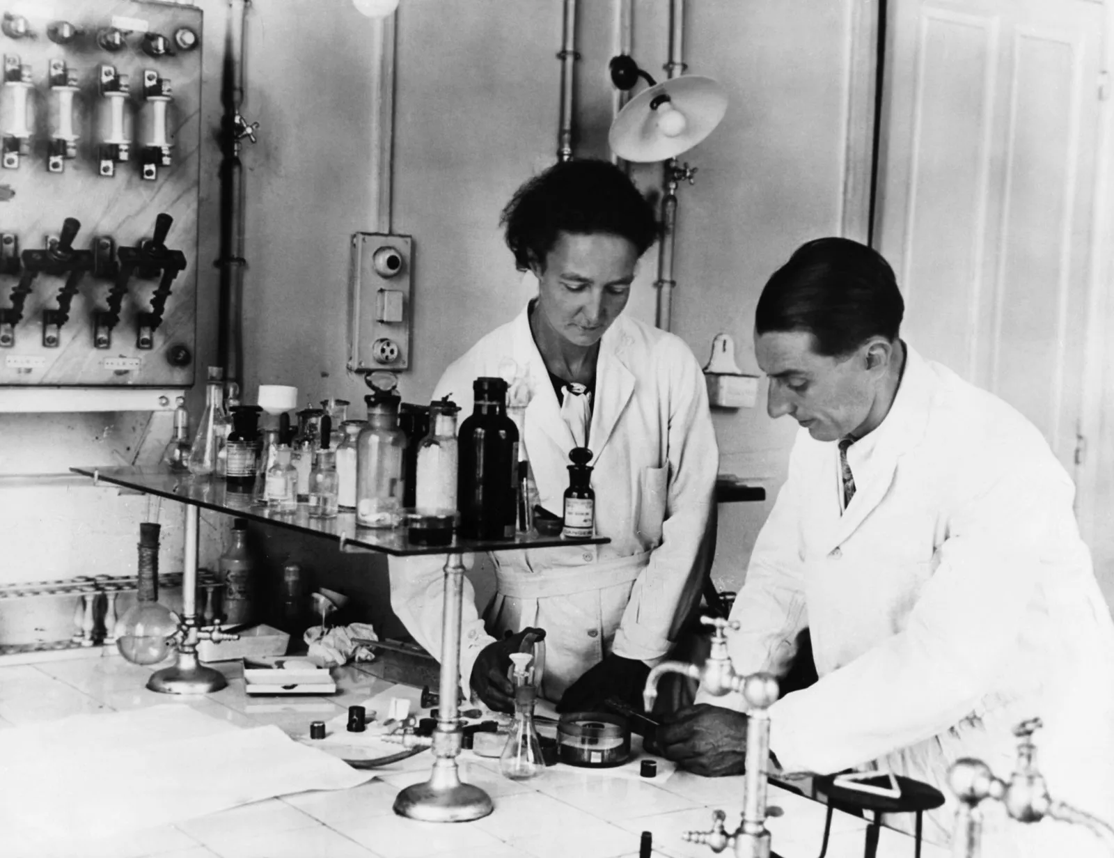
A black-and-white photograph of Irène and Frédéric Joliot-Curie working at a laboratory bench with glassware and an electrical switchboard behind them. — Irène and Frédéric Joliot-Curie in their Paris laboratory. Their 1934 discovery of artificial radioactivity was the first controlled observation of positron emission, and won the 1935 Nobel Prize in Chemistry.

The same decay happens across the Galaxy. Isotopes forged in supernovae — ²⁶Al, ⁴⁴Ti, ⁵⁶Co — are β⁺ emitters, and their positrons light up the 511 keV line: the brightest persistent gamma-ray line of cosmic origin, whose dominant source is still unidentified after fifty years.

A composite multi-wavelength image of Kepler's supernova remnant, an expanding shell of glowing gas and dust. — Kepler’s supernova remnant. Supernovae synthesise the β⁺-emitting isotopes that seed the Galaxy with positrons.

COSI, a NASA Small Explorer mission launching in 2027, will map that line with high-purity germanium (HPGe) detectors. The catch: cosmic rays activate the spacecraft itself into a background that also emits at 511 keV, and COSI’s analysis chain had no way to tag a β⁺ event — pipelines only ever vetoed them. BEvAn, the β⁺ Decay Event Analyzer, inverts that test. Built at UC Berkeley’s Space Sciences Laboratory with Andreas Zoglauer and John Tomsick; in preparation for the American Astronomical Society (AAS).

A dark-themed organizational chart of the COSI mission, grouping partner institutions by role: management and systems engineering, payload and instrument, electronics and flight software, spacecraft subsystems, integration and test, science and analysis, ground segment and operations, and launch. — COSI is led by UC Berkeley’s Space Sciences Laboratory with a consortium spanning instrument, spacecraft, science, and operations. Mapping the Galactic 511 keV line is one of its primary goals.

The signature — and everything that fakes it

An annihilation leaves a particular imprint in germanium: two photons Compton-scattering through the array, each recorded interaction a hit with a position and an energy. A clean event writes up to two scatter chains, with energies climbing toward 511 keV per photon and initial directions anti-parallel.

No single property is unique to annihilation, though. Compton-continuum events, partial deposits, and de-excitation gamma-rays each mimic one aspect of the signature — almost never all of them at once. The joint structure is what a real annihilation has and a background imitation lacks.

How it works

BEvAn never sees the decay, only the hits its photons leave behind. Three steps turn those into a decision: reconstruct the event, reduce it to three physically motivated scalars, and combine them through naive Bayes — chosen for transparency and for being cheap to refit as the in-orbit background drifts.

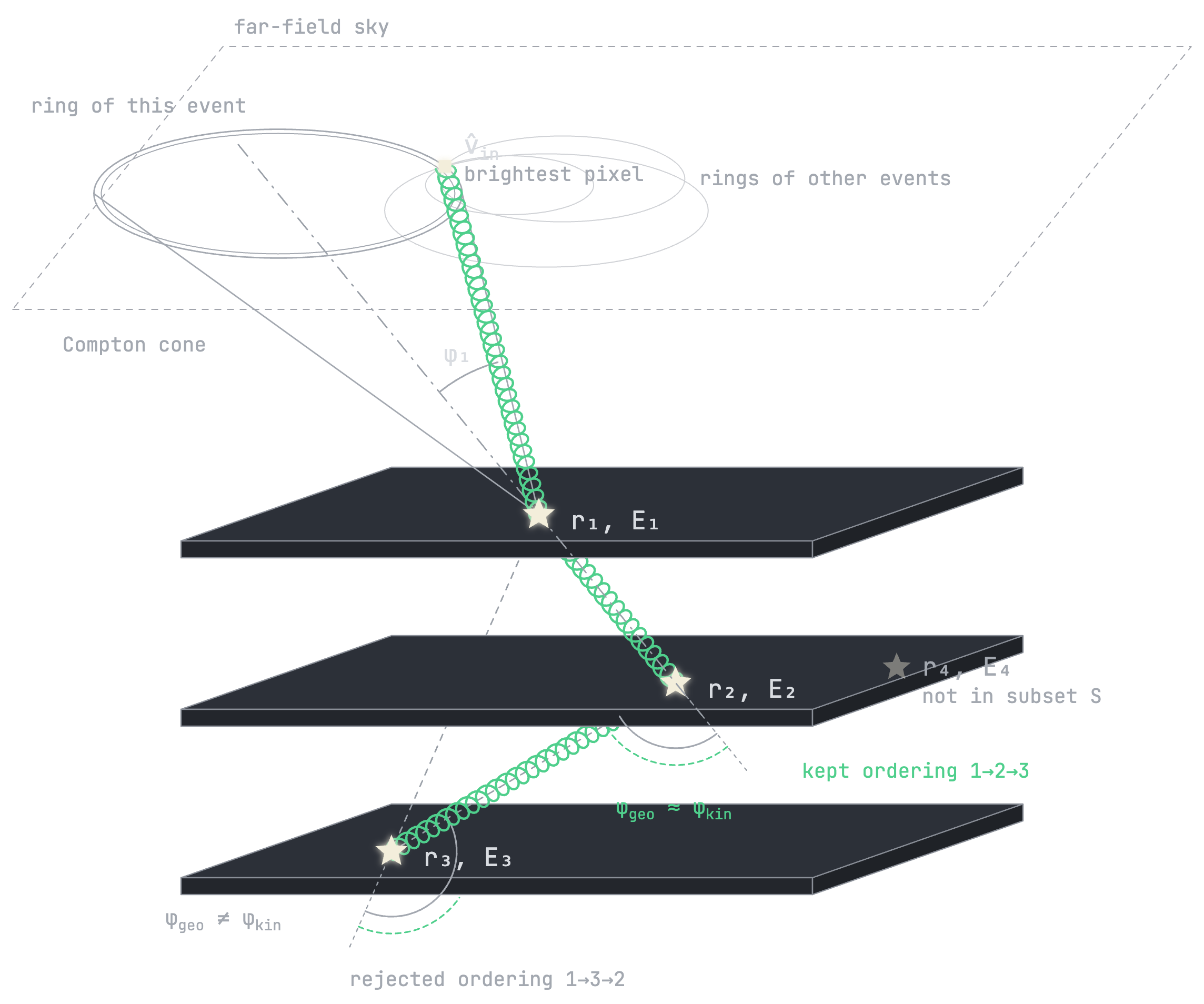
A 3D schematic of event reconstruction. A photon arrives from the far-field sky, Compton-scatters through three stacked detector planes at hits r1/E1, r2/E2, r3/E3, and its Compton cone projects a ring onto the sky. Rings from other events overlap at the brightest pixel, which fixes the incoming direction v-in. The ordering 1→2→3 is kept because the geometric and kinematic scatter angles agree; the ordering 1→3→2 is rejected because they disagree. A fourth hit r4/E4 is marked as not in the subset S. — Event reconstruction. Each event’s Compton cone draws a ring on the sky; the rings of many events overlap at the brightest pixel, which fixes the incoming direction v̂ᵢₙ. The hits’ interaction order is then chosen by demanding that the geometric scatter angle match the kinematic one from the energies.

The three physics factors. Each event is reduced to three scalars, each testing a different half of the signature and blind to what the others measure.

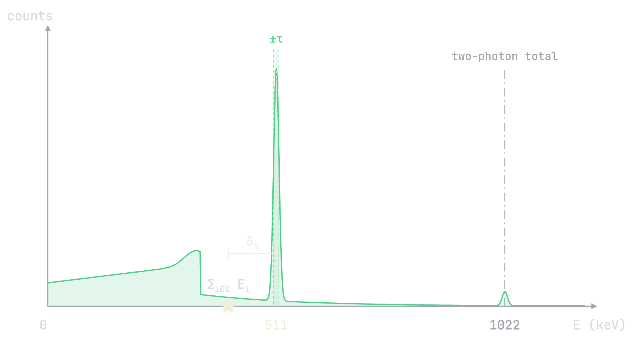
An energy spectrum in counts versus keV, showing a Compton continuum with its edge, a sharp photopeak at 511 keV with a tolerance band plus or minus tau around it, and a small peak at the 1022 keV two-photon total. A candidate's summed energy sits below the peak, its distance from 511 keV marked delta-S. — ΔE, the energy-consistency factor. How far a candidate’s summed deposit δ_S falls from the 511 keV line, relative to the detector’s tolerance ±τ. A fully absorbed annihilation photon lands near zero; the Compton continuum and partial deposits spread far from it.

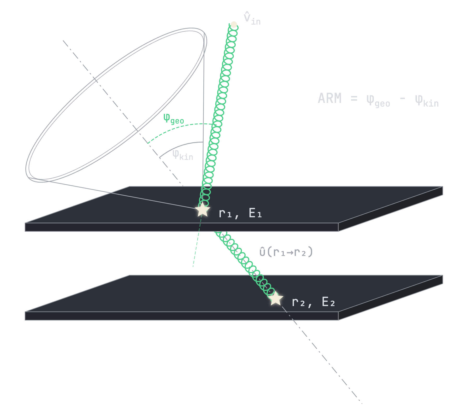
A 3D schematic of two detector planes. A photon arrives along v-in, scatters at r1/E1 and continues to r2/E2. The Compton cone opens around the scatter axis with kinematic half-angle psi-kin, while the geometric angle psi-geo is measured between the incoming direction and the r1-to-r2 segment. ARM equals psi-geo minus psi-kin. — Ω, the angular resolution measure (ARM) score. The gap between the scatter angle the geometry shows, ψ_geo, and the one the energies imply for a 511 keV photon, ψ_kin. A real annihilation photon from the reconstructed direction drives it to zero.

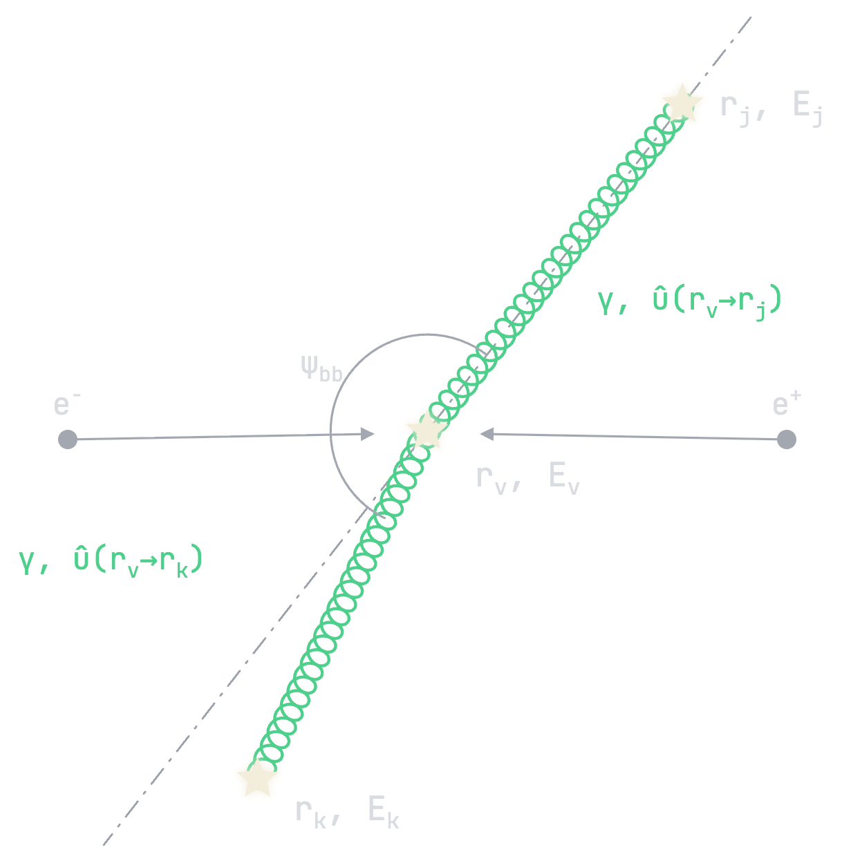
A diagram of an electron and a positron meeting at a vertex r-v, from which two photons leave along the directions v-to-r-j and v-to-r-k. The angle between the two arms is labelled psi-bb. — Ψ, the back-to-back score. Two photons leaving a common vertex in opposite directions, ψ_bb → 180°, is the one thing the other two factors miss — the defining mark of a pair.

Multiplicity classes. ΔE needs one hit, Ω a candidate of two, Ψ a vertex with two arms. Events are routed by how much their reconstruction produced, each class with its own densities and prior, so a missing factor is never imputed.

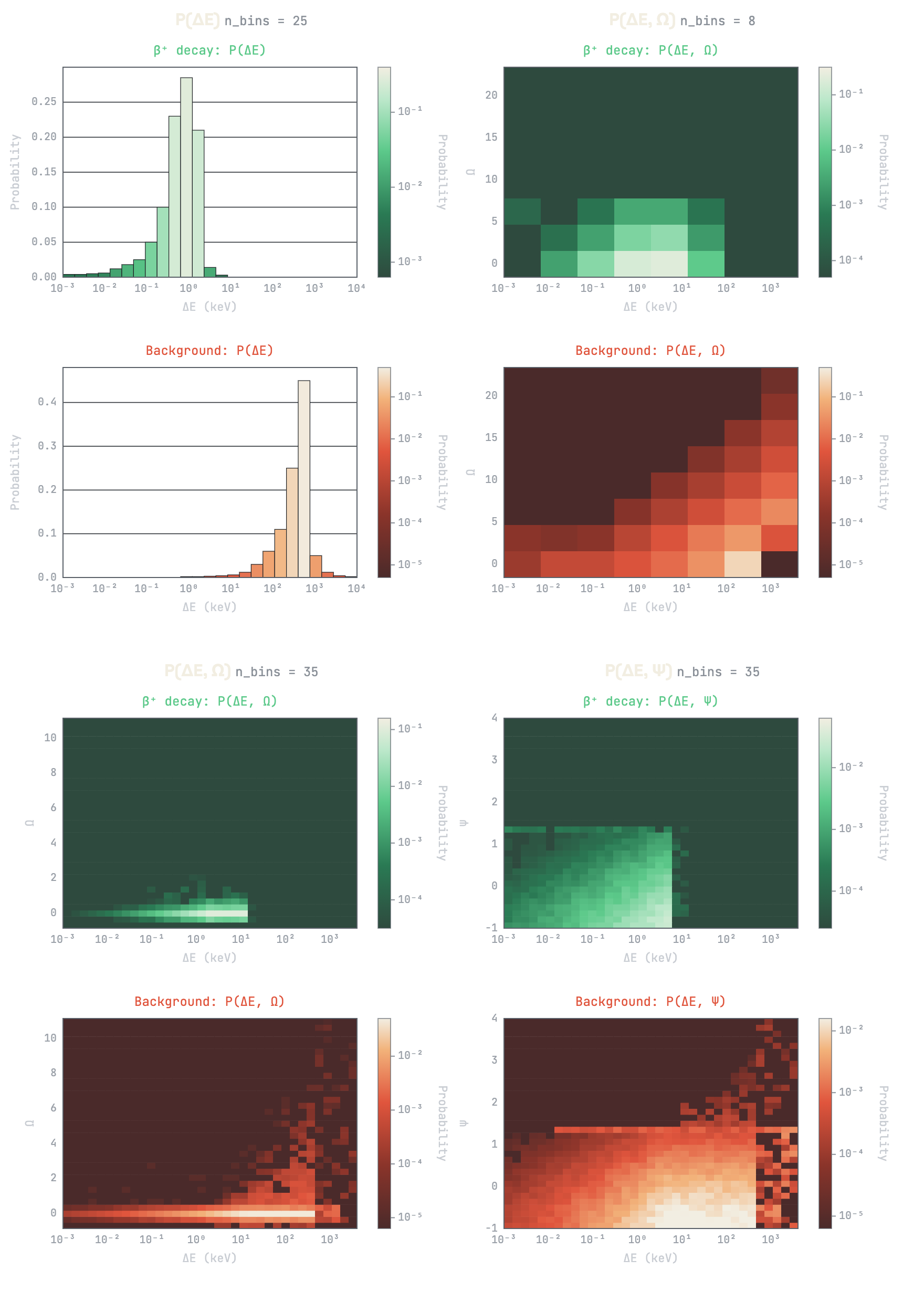
Densities, not thresholds. For each class and each of β⁺ and background, BEvAn estimates a smoothed 2D histogram over the feature space, pairing the angular scores with ΔE to keep their correlation. The ratio of the two densities in an event’s cell is its likelihood ratio. Empty cells get a small Jeffreys pseudo-count; the ΔE axis is log-spaced so the region near zero is finely resolved.

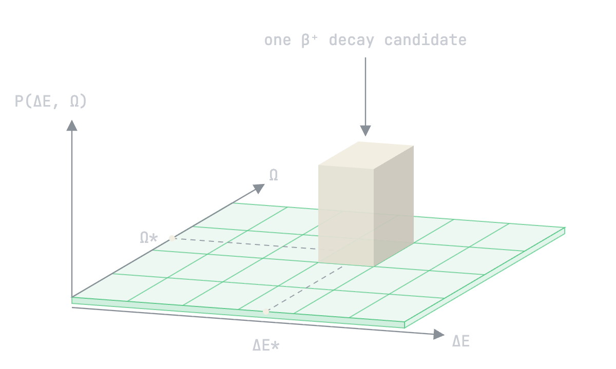
A 3D illustration of a class-conditional density matrix. A green grid spans two axes, delta-E and Omega, with probability on the vertical axis. One cell is raised into a tall bar, marking where a single beta-plus decay candidate falls. — Constructing a class-conditional density. Training events are bucketed into a grid over (ΔE, Ω); the highlighted bar is where one β⁺ candidate lands and the value BEvAn reads off.

An eight-panel grid of class-conditional density matrices. Top rows are the beta-plus decay class in green, bottom rows the background class in orange-red. Beta-plus mass concentrates at low delta-E and low angular score; background spreads across the full plane. — The learned densities for the twelve-detector COSI balloon, one panel per term. β⁺ events (green) pile up at low ΔE and low angular score; background (orange) fills the plane. This is BEvAn’s hardest of the seven geometries.

The decision. Naive Bayes multiplies each class’s density terms with a prior and assigns the larger posterior. Equivalently, a single evidence sum: log-likelihood ratios weighed against log prior odds — separately readable terms that show what each factor contributed.

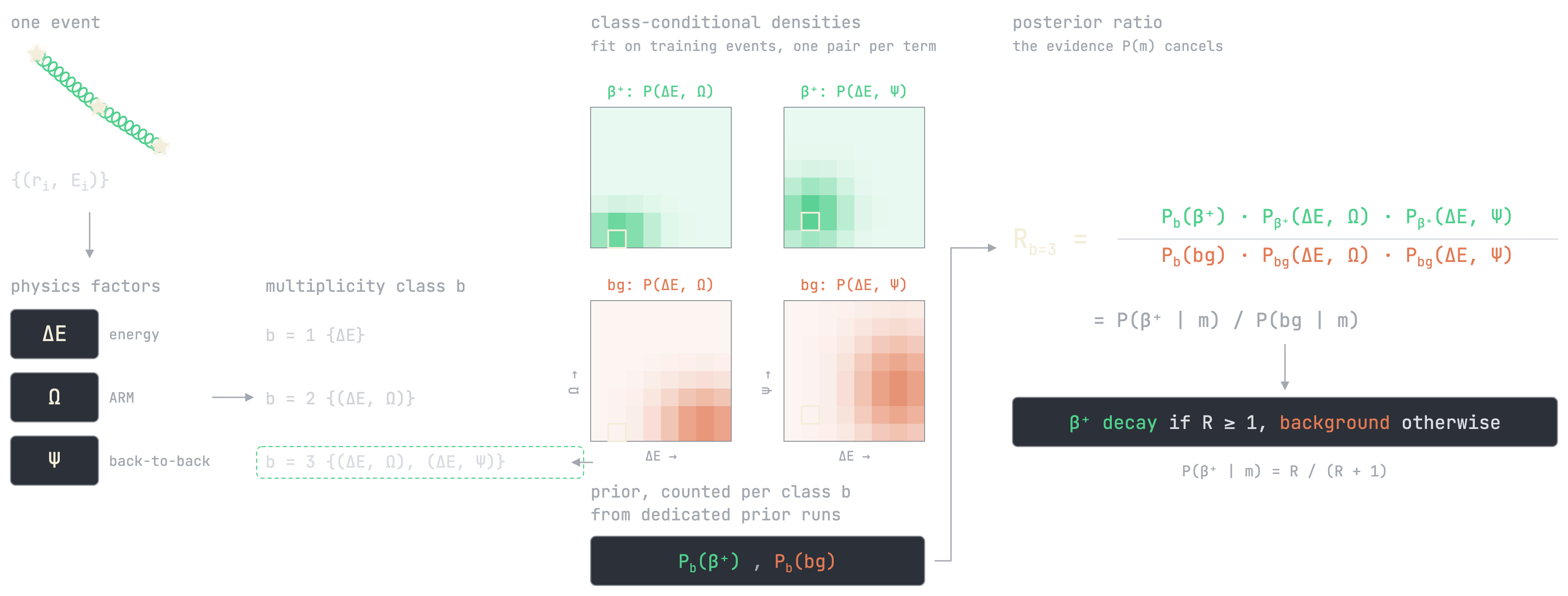
A left-to-right pipeline diagram. One event's hits become three physics factors, delta-E, Omega, and Psi, which route the event into multiplicity class b = 1, 2, or 3. Class-conditional density matrices over (delta-E, Omega) and (delta-E, Psi) are shown for the beta-plus class in green and the background class in orange, with the event's cell highlighted in each. Together with per-class priors, they form the posterior ratio R as a product of prior and density terms, and the decision reads beta-plus decay if R is at least 1, background otherwise. — The full pipeline for one event. Hits become the three physics factors, which fix the multiplicity class; the event’s cell is read off each class-conditional density, multiplied with the per-class prior, and the posterior ratio R decides: β⁺ decay if R ≥ 1, background otherwise.

Results

Trained and evaluated on MEGAlib activation simulations of seven HPGe geometries, from a four-layer telescope to a 125-detector array. The separation is a property of the annihilation signature, not the instrument: ROC-AUC spans just 98.3–99.6 % across a thirtyfold change in detector count.

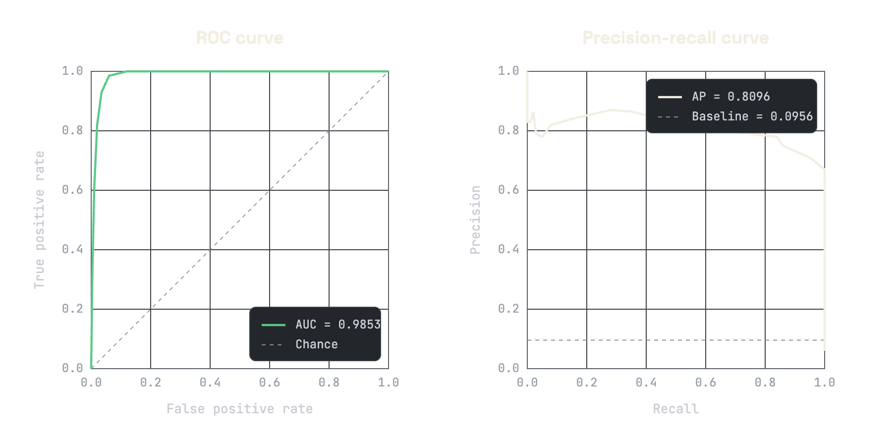
Two plots side by side. Left, an ROC curve rising almost immediately to the top-left corner against a dashed chance diagonal. Right, a precision-recall curve holding high precision across most of the recall range. — ROC and precision–recall for the twelve-detector COSI balloon, close to BEvAn’s worst case. β⁺ events are only a few percent of the sample.

BEvAn recovers roughly 90–97 % of true β⁺ events at 80–85 % precision — tuned toward completeness, because for annihilation-line science the expensive mistake is discarding a real event, not admitting a few extra.

The obvious heuristic is a single cut: tag an event β⁺ if its total energy falls near 511 keV. At the heuristic’s own false-positive rate, BEvAn beats it on both precision and recall in every geometry, with the widest margin on complex, high-multiplicity instruments where several photons pile into one event and an energy sum can no longer isolate the annihilation photon. Where energy alone nearly suffices, the angular factors add little; where deposits pile together, they carry the physics the energy test has lost.

It is also cheap. Nearly all the cost is building the factors, at a few hundred microseconds to two milliseconds per event; scoring runs at order 10⁷ events per second, and the fitted model is 25 kB — small enough to refit epoch by epoch as the activation background builds after each pass through the South Atlantic Anomaly.

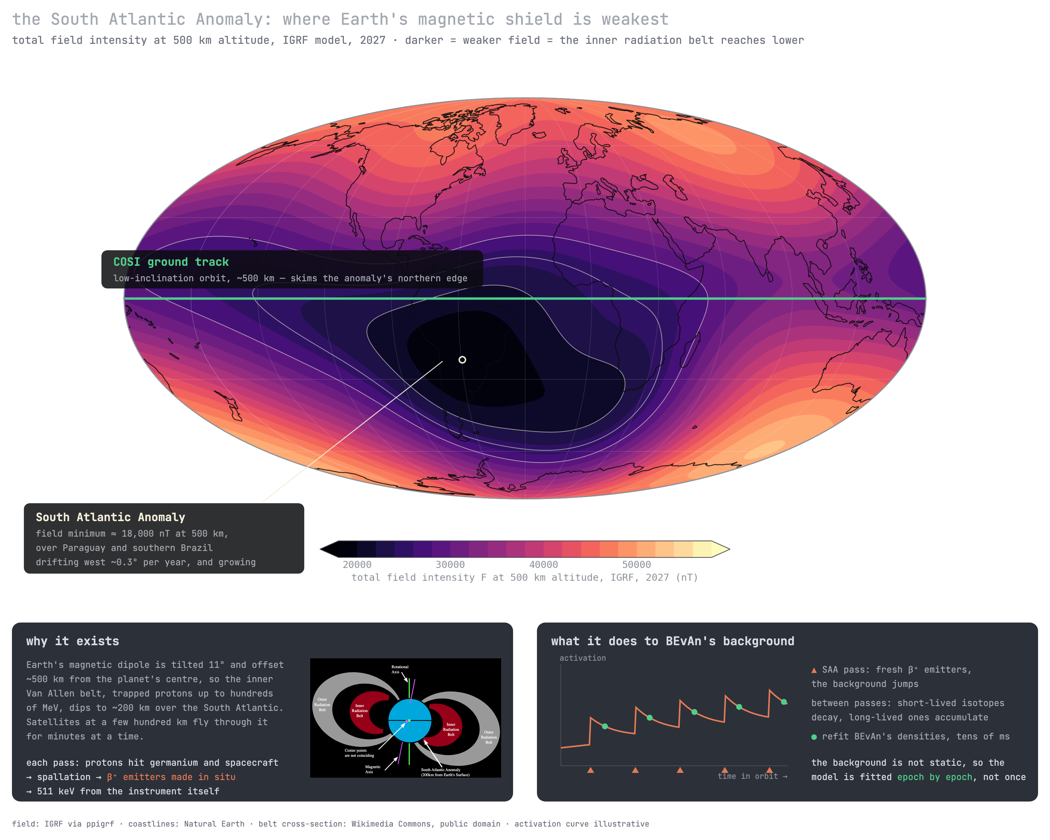
A Mollweide map of Earth's total magnetic field intensity at 500 km altitude from the IGRF model for 2027, with coastlines. The field is weakest in a dark region over southern Brazil, Paraguay, and the South Atlantic, the South Atlantic Anomaly, with a marked minimum near 18,000 nT; COSI's near-equatorial ground track is drawn in green skimming the anomaly's northern edge. Below: a cross-section of the Van Allen belts showing the tilted, offset magnetic axis and the inner belt dipping to 200 km, and an activation-versus-time curve that jumps at each SAA pass and decays between, with markers where BEvAn's densities are refit. — The South Atlantic Anomaly. Earth’s magnetic dipole is tilted and offset from the planet’s centre, so the field is weakest over the South Atlantic and the inner radiation belt dips to about 200 km there. COSI’s low-inclination orbit minimises time inside it, but every pass still makes fresh β⁺ emitters in the germanium and spacecraft, so the 511 keV background BEvAn separates keeps moving. That is why the model is built to be refit epoch by epoch rather than fitted once. Field from the IGRF model; belt cross-section from Wikimedia Commons.

What I took away

The difficulty lives in the physics factors, not the inference. Nearly all of the signal, and nearly all of the cost, is in building the Compton reconstruction, the scatter kinematics, and the back-to-back geometry; the classifier on top is a deliberately simple, readable sum.

That points to the next step. An event is already a graph — hits as nodes, kinematic relations as edges — and the current pipeline collapses it into three scalars. A graph neural network could score the hit structure directly, at the price of a larger model and the per-factor transparency. The way to get both is to stack them: BEvAn runs first as a cheap, high-recall filter that hands on a β⁺-enriched pool, and a GNN then rejects the residual background it cannot separate. Since the second stage only removes candidates, BEvAn sets the recall ceiling and the GNN buys precision.

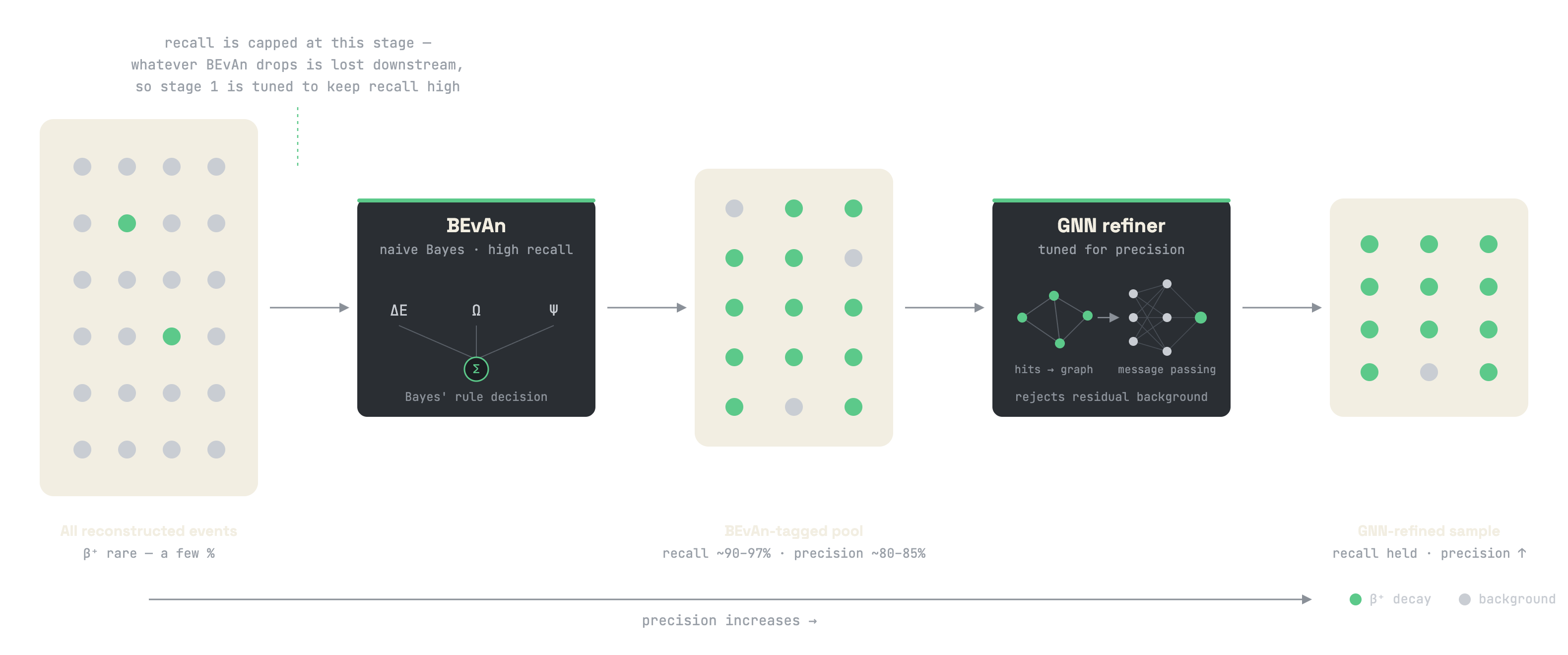
A two-stage cascade diagram. A pool of mostly grey dots with a few green ones enters a box labelled BEvAn, naive Bayes, high recall, which outputs a smaller mostly-green pool. That enters a box labelled GNN refiner, tuned for precision, whose output is almost all green dots. — The proposed cascade. BEvAn shrinks the stream to a β⁺-enriched pool without dropping real events; a GNN then refines it for purity. Completeness from stage one, purity from stage two.